
Concept Demonstrations
Waves through a locally resonant metamaterial
A chain of twelve unit cells sits between two non-dispersive media. Choose a frequency and see whether vibration crosses the chain, and how fast its phase and energy travel.
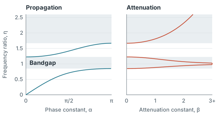
Drag the frequency line on the plots, or use the slider. On the left plot, the slope of the line from the origin gives the phase velocity, and the slope of the tangent gives the group velocity (plot axes are not to equal scale). The motion is drawn vertically, and resonator motion is capped for display.
Formulation
This follows the negative mass (NM) monocoupled system and the method of Bhatt, Banerjee and Adhikari (2022), obtained from its generalised system by setting \(m_a=0\) and \(m_2=0\), with \(m_1\), \(k_1\), \(\theta_{r1}\), \(\eta_{r1}\) and \(\zeta_{r1}\) written as \(m\), \(k\), \(\theta_r\), \(\eta_r\) and \(\zeta_r\).
1. Unit cell and dynamic stiffness
Main-chain masses \(M\) at nodes 1 and 4 are joined by a spring \(K\). Each carries a resonator \(m\) (nodes 2 and 3) through a spring \(k\). The equations of motion are

With \(\ddot{(\bullet)}=-\omega^2(\bullet)\), condensing out nodes 2 and 3 gives the dynamic stiffness matrix, and its inverse gives the receptance matrix:
2. Dispersion relation
Bloch's theorem relates the left and right displacements and forces through the propagation constant \(\kappa=\alpha+i\beta\):
The wave propagates with \(\alpha=\cos^{-1}x\) and \(\beta=0\) when \(x^2\lt 1\). When \(x^2\gt 1\) it attenuates, with \(\alpha=\pi\) for \(x\lt -1\), \(\alpha=0\) for \(x\gt 1\), and \(\beta=\cosh^{-1}|x|\).
3. Peak and bounds of the attenuation band
Using \(\eta=\omega/\sqrt{K/M}\), \(\theta_r=m/M\) and \(\eta_r=\sqrt{k/m}/\sqrt{K/M}\), the dispersion relation takes the rational form
The attenuation peak is at \(Q=0\), and the band boundaries are at \(R=0\) (\(\kappa=0\)) and \(R+2Q=0\) (\(\kappa=\pi\), the Bragg condition):
The demonstration uses \(\theta_r=0.5\) and \(\eta_r=1\). The Bragg boundaries are then \(\eta_B=0.848\) and \(1.668\), the peak is at \(\eta=1\), and \(\zeta_r=1.225\).
Velocity formulation
In a propagation band, with \(L\) the cell length, the velocities in units of \(L\sqrt{K/M}\) follow from \(\cos\alpha=g(\eta^2)\):
\(\sin\alpha\) vanishes at both \(\kappa=0\) and \(\kappa=\pi\), so \(c_g=0\) at every band boundary, while \(c_p\) stays finite at the Bragg boundary. Solving \(\cos\kappa=g(\eta^2)\) gives each band exactly, with the minus sign for the lower band and the plus sign for the upper band:
The wave packet panel is an exact sum of Bloch waves with a Gaussian spectrum of width \(\sigma_\kappa\), so it includes dispersive spreading:
Impedance formulation
From the receptance relation and Bloch's theorem, with \(D=K\cos\kappa\), the force at the left node of the cell is
Dividing force by velocity amplitude gives the Bloch impedance of a propagating wave:
This value applies when the cell boundary passes through the node masses, as in this unit cell. It depends on where the boundary is placed. In the long-wave limit, it gives the impedance chosen for the two media:
Finite chain between the two media
The media are semi-infinite, so their far ends do not reflect. For incident, reflected and transmitted amplitudes \(U_I\), \(U_R\) and \(U_T\), with \(\kappa_0\) the wavenumber per cell and \(n\) measured from each interface:
Assembling \(N=12\) cells gives a tridiagonal system for the node displacements \(d_0\) to \(d_N\):
In a propagation band this solves to the closed form
What happens at the band edges
\(Z_B\to0\) and \(c_g\to0\) at a band boundary. Taking this limit at \(\eta_B\) gives a transmission that is small but not zero, and falls as \(1/N\) instead of exponentially:
For this chain that is 11% at \(\eta=0.848\) and 6% at \(\eta=1.668\). The infinite-chain band edge is sharp, but a finite chain has only a gradual transition around it. The impedance mismatch also reflects most of the wave just inside the band, so a finite chain is not a sharp switch at this frequency.
References
- A. Bhatt, A. Banerjee and S. Adhikari, Closed-form solutions for attenuation peaks and band boundaries of general monocoupled systems, Journal of Sound and Vibration, 541, 117318, 2022.
- L. Brillouin, Wave Propagation in Periodic Structures, McGraw-Hill, 1946.
- M. I. Hussein, M. J. Leamy and M. Ruzzene, Dynamics of phononic materials and structures: Historical origins, recent progress, and future outlook, Applied Mechanics Reviews, 66, 040802, 2014.
- D. J. Colquitt, R. V. Craster and M. Makwana, High frequency homogenisation for elastic lattices, on behaviour close to band edges.